MobileNet V1

MobileNets: Efficient Convolutional Neural Networks for Mobile Vision Applications

Andrew G. Howard, Menglong Zhu, Bo Chen, Dmitry Kalenichenko, Weijun Wang, Tobias Weyand, Marcj Andreetto, Hartwig Adam
Google Inc.

[Introduction]

• Propose a streamlined architecture that uses depthwise separable convolutions to build light weight deep neural networks and two simple global hyperparameters that efficiently trade off between latency and accuracy
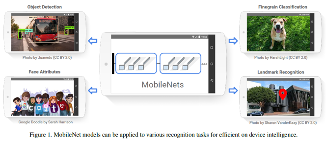
• A class of efficient models called MobileNets for mobile and embedded vision applications
• Focus on optimizing for latency but also yield small networks

  • Many papers on small networks focus only on size but do not consider

    

[MobileNet Architecture]

1. Depthwise Separable Convolution

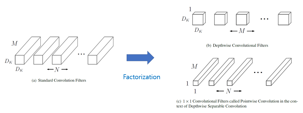
The MobileNet model is based on depthwise separable convolutions which is a form of factorized convolutions which factorize a standard convolution into a depthwise convolution and a 1x1 convolution called a pointwise convolution

• Standard convolution -> Depthwise convolution + Pointwise convolution
• Depthwise convolution
  Apply a single filter to each input channel
• Pointwise convolution
  1x1 convolution to combine the outputs the depthwise convolution
• Computational cost
  Standard convolution: D_K x D_K x M x N x D_F x D_F

  depends multicatively on the number of input channels, the number of output channels, the kernel size and the feature map size

  Depthwise separable convolution: D_K x D_K x M x D_F x D_F + M x N x D_F x D_F

  • D_K: spatial width, height of a kernel
  • D_F: spatial width, height of a square input feature map
  • M: number of input channels

  • N: number of output channels

    

2. Network Structure and Training

• The MobileNet structure is built on depthwise separable convolutions as mentioned in the previous section except for the first layer which is a full convolution
• All layers are followed by a batchnorm and ReLU nonlinearity with the exception of the final fully connected layer which has no nonlinearity and feeds into a softmax layer for classification
• A final average pooling reduces the spatial resolution to 1 before the finally connected layer

• Counting depthwise and pointwise convolutions as separable layers, MobileNet has 28 layers

  </img>

It is important not only small number of Mult-Adds but also operations that can be efficiently implementable

Unstructured sparse matrix operations are not typically faster than dense matrix operations until a very high level of sparsity

• MobileNet model structure puts nearly all of the computation into dense 1x1 convolutions
• Can be implented with highly optimized general matrix multiply(GEMM) functions
• Often convolutions are implementaed by a GEMM require an initial reordering in memory called im2col in order to map it to a GEMM
• 1x1 convolution do not require this reordering in memory and can be implemented directly with GEMM which is one of the most optimized numerical linear algebra algorithms (Contrary to training large models)
• Use less regularization and data augmentation techniques because small models have less trouble with overfitting

3. Width Multiplier: Thinner Models

Although the base MobileNet architecture is already small and low latency, many times a specific use case or application may require the model to be smaller and faster

• In order to construct smaller and less computationally expensive models, introduce a parameter 𝛼
• The role of the width multiplier &alpha is to thin a network uniformly at each layer
• For a given layer and width multiplier &alpha, the number of input channels M becomes \alpha M and the numver of output channels N becomes 𝛼N

• Computational Cost of a depthwise separable convolution with width multiplier &alpha

  D_K x D_K x 𝛼M x D_F x D_F + 𝛼M x 𝛼N x D_F x D_F

• Width multiplier has the effect of reducing computational cost and the number of parameters quadratically by roughly 𝛼²

4. Resolution Multiplier: Reduced Representation

• The second hyperparameter to reduce the computational cost of a neural network is a resolution multiplier 𝜌
• Apply 𝜌 to input image and the internal representation of every layer is subsequently reduced by the same multiplier

• Computational cost of the core layers of network as depthwise separable convolutions with width multiplier 𝛼 and resolution multiplier 𝜌

  D_K x D_K x 𝛼M x 𝜌D_F x 𝜌D_F + 𝛼M x 𝛼N x 𝜌D_F x 𝜌D_F where 𝜌 which is typically set implicitly so that the input resolution of the network is 224, 192, 160 or 128

• Resolution multiplier has the effect of reducing computational cost by 𝜌²

[Experiments]

• Model choices
• Model shrinking hyperparameters